Tutorial 2b: Single-Point Visualizations
Contents
Tutorial 2b: Single-Point Visualizations#
This tutorial is an introduction to analyzing results from a single-point simulation. It uses results from the case you ran in the 2a Tutorial, but you don’t have to wait for those runs to complete before doing this tutorial too. We’ve prestaged model results from this simulation in a shared directory. This way, you can get started on analyzing simulations results before your simulations finish running. We also ran this case for longer (10 years instead of 1), so that we have more data to work with.
In this tutorial#
The tutorial has several objectives:
Increase familiarity with Jupyter Notebooks
Increase knowledge of python packages and their utilities
Visualize output from a single-point CTSM simulation.
As in other visualization notebook, this should be run in a Python3 kernel
We’ll start by loading some packages
import os

import xarray as xr
import functools
import numpy as np
import matplotlib.pyplot as plt

%matplotlib inline
NOTE: This example largely uses features of xarray and matplotlib packages. We won’t go into the basics of python or features in these packages, but there are lots of resources to help get you started. Some of these are listed below.
NCAR python tutorial, which introduces python, the conda package manager, and more on github.
NCAR ESDS tutorial series, features several recorded tutorials on a wide variety of topics.
GeoCAT examples, with some nice plotting examples
1. Reading and formatting data#
1.1 Find the correct directories and file names#
path = '/scratch/data/day2/'       # path to archived simulations
case = 'I2000_CTSM_singlept'       # case name
years = list(range(2001, 2011, 1)) # look at 10 years of data (python won't count the last year in the list, here 2011)
months = list(range(1, 13, 1))     # we want all months (again, python will go up to, but not including month 13)

# build a list of file names based on the year and month
file_names = [f"{case}.clm2.h0.{str(year)}-{str(month).rjust(2, '0')}.nc"
              for year in years for month in months]

# create their full path
full_paths = [os.path.join(path, case, 'lnd/hist', fname) for fname in file_names]

# print the last file in our list
print(full_paths[-1])
/scratch/data/day2/I2000_CTSM_singlept/lnd/hist/I2000_CTSM_singlept.clm2.h0.2010-12.nc
Typically we post-process these data to generate single variable time series for an experiment. This means that the full time series of model output for each variable, like rain, air temperature, or latent heat flux, are each in their own file. A post-processing tutorial will be available at a later date, but for now we'll just read in the monthly history files described above.
1.2 Open files & load variables#
This is done with the xarray function open_mfdataset
To make this go faster, we’re going to preprocess the data so we’re just reading the variables we want to look at.
As in our Day 1 tutorial, we will begin by looking at ‘all sky albedo’, which is the ratio of reflected to incoming solar radiation (FSR/FSDS). Other intereresting variables might include latent heat flux (EFLX_LH_TOT) or gross primary productivity (GPP).
# define the history variables to read in
fields = ['FSR', 'FSDS', 'GPP', 'EFLX_LH_TOT', 'FCEV', 'FCTR', 'FGEV', 'ELAI',
          'H2OSOI', 'HR', 'TBOT', 'TSOI']


def preprocess(ds, fields):
    '''Selects the variables we want to read in
       Drops lndgrid because we are on a single point'''

    return ds[fields].sel(lndgrid=0)


def fix_time(ds):
    '''Does a quick fix to adjust time vector for monthly data'''
    nmonths = len(ds.time)
    yr0 = ds['time.year'][0].values
    ds['time'] = xr.cftime_range(str(yr0), periods=nmonths, freq='MS')

    return ds


# open the dataset -- this may take a bit of time
ds = fix_time(xr.open_mfdataset(full_paths, decode_times=True,
                                preprocess=functools.partial(preprocess, fields=fields)))

print('-- your data have been read in -- ')
-- your data have been read in --
Printing information about the dataset is helpful for understanding your data.
What dimensions do your data have?
What are the coordinate variables?
What variables are we looking at?
Is there other helpful information, or are there attributes in the dataset we should be aware of?
# This cell will print information about the dataset
ds
<xarray.Dataset>
Dimensions:      (time: 120, levsoi: 20, levgrnd: 25)
Coordinates:
  * levgrnd      (levgrnd) float32 0.01 0.04 0.09 0.16 ... 19.48 28.87 42.0
  * levsoi       (levsoi) float32 0.01 0.04 0.09 0.16 ... 5.06 5.95 6.94 8.03
  * time         (time) object 2001-01-01 00:00:00 ... 2010-12-01 00:00:00
Data variables:
    FSR          (time) float32 dask.array<chunksize=(1,), meta=np.ndarray>
    FSDS         (time) float32 dask.array<chunksize=(1,), meta=np.ndarray>
    GPP          (time) float32 dask.array<chunksize=(1,), meta=np.ndarray>
    EFLX_LH_TOT  (time) float32 dask.array<chunksize=(1,), meta=np.ndarray>
    FCEV         (time) float32 dask.array<chunksize=(1,), meta=np.ndarray>
    FCTR         (time) float32 dask.array<chunksize=(1,), meta=np.ndarray>
    FGEV         (time) float32 dask.array<chunksize=(1,), meta=np.ndarray>
    ELAI         (time) float32 dask.array<chunksize=(1,), meta=np.ndarray>
    H2OSOI       (time, levsoi) float32 dask.array<chunksize=(1, 20), meta=np.ndarray>
    HR           (time) float32 dask.array<chunksize=(1,), meta=np.ndarray>
    TBOT         (time) float32 dask.array<chunksize=(1,), meta=np.ndarray>
    TSOI         (time, levgrnd) float32 dask.array<chunksize=(1, 25), meta=np.ndarray>
Attributes: (12/37)
    title:                                CLM History file information
    comment:                              NOTE: None of the variables are wei...
    Conventions:                          CF-1.0
    history:                              created on 05/19/22 14:47:50
    source:                               Community Terrestrial Systems Model
    hostname:                             cheyenne
    ...                                   ...
    ctype_urban_shadewall:                73
    ctype_urban_impervious_road:          74
    ctype_urban_pervious_road:            75
    cft_c3_crop:                          1
    cft_c3_irrigated:                     2
time_period_freq: month_1You can also print information about the variables in your dataset. The example below prints information about one of the data variables we read in. You can modify this cell to look at some of the other variables in the dataset.
What are the units, long name, and dimensions of your data?
ds.FSDS
<xarray.DataArray 'FSDS' (time: 120)>
dask.array<concatenate, shape=(120,), dtype=float32, chunksize=(1,), chunktype=numpy.ndarray>
Coordinates:
  * time     (time) object 2001-01-01 00:00:00 ... 2010-12-01 00:00:00
Attributes:
    long_name:      atmospheric incident solar radiation
    units:          W/m^2
    cell_methods:   time: mean
landunit_mask: unknownds.ASA) or using brackets with the variable or coordinates in quotes ( ds['ASA']).
1.3 Adding derived variables to the dataset#
As in Day 1, we will calculate the all sky albedo (ASA). Remember from above that this is the ratio of reflected to incoming solar radiation (FSR/FSDS).
We will add this as a new variable in the dataset (which requires using quotes; e.g., ds['ASA']) and add appropriate metadata.
When doing calculations, it is important to avoid dividing by zero. Use the .where function for this purpose
ds['ASA'] = ds.FSR/ds.FSDS.where(ds.FSDS > 0.0)
ds['ASA'].attrs['units'] = 'unitless'
ds['ASA'].attrs['long_name'] = 'All sky albedo'
2. Filtering and indexing data#
xarray allows for easy subsetting and filtering using the .sel and .isel functions. .sel filters to exact (or nearest neighbor) values, whereas .isel filters to an index.
Let’s filter to a specific date. Note that because our output was monthly and at one latitude and longitude point, this should only give us one point of data.
# filter to specific date
ds.sel(time="2001-01-01")
<xarray.Dataset>
Dimensions:      (time: 1, levsoi: 20, levgrnd: 25)
Coordinates:
  * levgrnd      (levgrnd) float32 0.01 0.04 0.09 0.16 ... 19.48 28.87 42.0
  * levsoi       (levsoi) float32 0.01 0.04 0.09 0.16 ... 5.06 5.95 6.94 8.03
  * time         (time) object 2001-01-01 00:00:00
Data variables: (12/13)
    FSR          (time) float32 dask.array<chunksize=(1,), meta=np.ndarray>
    FSDS         (time) float32 dask.array<chunksize=(1,), meta=np.ndarray>
    GPP          (time) float32 dask.array<chunksize=(1,), meta=np.ndarray>
    EFLX_LH_TOT  (time) float32 dask.array<chunksize=(1,), meta=np.ndarray>
    FCEV         (time) float32 dask.array<chunksize=(1,), meta=np.ndarray>
    FCTR         (time) float32 dask.array<chunksize=(1,), meta=np.ndarray>
    ...           ...
    ELAI         (time) float32 dask.array<chunksize=(1,), meta=np.ndarray>
    H2OSOI       (time, levsoi) float32 dask.array<chunksize=(1, 20), meta=np.ndarray>
    HR           (time) float32 dask.array<chunksize=(1,), meta=np.ndarray>
    TBOT         (time) float32 dask.array<chunksize=(1,), meta=np.ndarray>
    TSOI         (time, levgrnd) float32 dask.array<chunksize=(1, 25), meta=np.ndarray>
    ASA          (time) float32 dask.array<chunksize=(1,), meta=np.ndarray>
Attributes: (12/37)
    title:                                CLM History file information
    comment:                              NOTE: None of the variables are wei...
    Conventions:                          CF-1.0
    history:                              created on 05/19/22 14:47:50
    source:                               Community Terrestrial Systems Model
    hostname:                             cheyenne
    ...                                   ...
    ctype_urban_shadewall:                73
    ctype_urban_impervious_road:          74
    ctype_urban_pervious_road:            75
    cft_c3_crop:                          1
    cft_c3_irrigated:                     2
time_period_freq: month_1We can also filter to a date range using the .slice function.
# filter by a date range
ds.sel(time=slice('2001-01-01', '2001-06-01'))
<xarray.Dataset>
Dimensions:      (time: 6, levsoi: 20, levgrnd: 25)
Coordinates:
  * levgrnd      (levgrnd) float32 0.01 0.04 0.09 0.16 ... 19.48 28.87 42.0
  * levsoi       (levsoi) float32 0.01 0.04 0.09 0.16 ... 5.06 5.95 6.94 8.03
  * time         (time) object 2001-01-01 00:00:00 ... 2001-06-01 00:00:00
Data variables: (12/13)
    FSR          (time) float32 dask.array<chunksize=(1,), meta=np.ndarray>
    FSDS         (time) float32 dask.array<chunksize=(1,), meta=np.ndarray>
    GPP          (time) float32 dask.array<chunksize=(1,), meta=np.ndarray>
    EFLX_LH_TOT  (time) float32 dask.array<chunksize=(1,), meta=np.ndarray>
    FCEV         (time) float32 dask.array<chunksize=(1,), meta=np.ndarray>
    FCTR         (time) float32 dask.array<chunksize=(1,), meta=np.ndarray>
    ...           ...
    ELAI         (time) float32 dask.array<chunksize=(1,), meta=np.ndarray>
    H2OSOI       (time, levsoi) float32 dask.array<chunksize=(1, 20), meta=np.ndarray>
    HR           (time) float32 dask.array<chunksize=(1,), meta=np.ndarray>
    TBOT         (time) float32 dask.array<chunksize=(1,), meta=np.ndarray>
    TSOI         (time, levgrnd) float32 dask.array<chunksize=(1, 25), meta=np.ndarray>
    ASA          (time) float32 dask.array<chunksize=(1,), meta=np.ndarray>
Attributes: (12/37)
    title:                                CLM History file information
    comment:                              NOTE: None of the variables are wei...
    Conventions:                          CF-1.0
    history:                              created on 05/19/22 14:47:50
    source:                               Community Terrestrial Systems Model
    hostname:                             cheyenne
    ...                                   ...
    ctype_urban_shadewall:                73
    ctype_urban_impervious_road:          74
    ctype_urban_pervious_road:            75
    cft_c3_crop:                          1
    cft_c3_irrigated:                     2
time_period_freq: month_1You can also filter to a whole year:
ds.sel(time='2001')
<xarray.Dataset>
Dimensions:      (time: 12, levsoi: 20, levgrnd: 25)
Coordinates:
  * levgrnd      (levgrnd) float32 0.01 0.04 0.09 0.16 ... 19.48 28.87 42.0
  * levsoi       (levsoi) float32 0.01 0.04 0.09 0.16 ... 5.06 5.95 6.94 8.03
  * time         (time) object 2001-01-01 00:00:00 ... 2001-12-01 00:00:00
Data variables: (12/13)
    FSR          (time) float32 dask.array<chunksize=(1,), meta=np.ndarray>
    FSDS         (time) float32 dask.array<chunksize=(1,), meta=np.ndarray>
    GPP          (time) float32 dask.array<chunksize=(1,), meta=np.ndarray>
    EFLX_LH_TOT  (time) float32 dask.array<chunksize=(1,), meta=np.ndarray>
    FCEV         (time) float32 dask.array<chunksize=(1,), meta=np.ndarray>
    FCTR         (time) float32 dask.array<chunksize=(1,), meta=np.ndarray>
    ...           ...
    ELAI         (time) float32 dask.array<chunksize=(1,), meta=np.ndarray>
    H2OSOI       (time, levsoi) float32 dask.array<chunksize=(1, 20), meta=np.ndarray>
    HR           (time) float32 dask.array<chunksize=(1,), meta=np.ndarray>
    TBOT         (time) float32 dask.array<chunksize=(1,), meta=np.ndarray>
    TSOI         (time, levgrnd) float32 dask.array<chunksize=(1, 25), meta=np.ndarray>
    ASA          (time) float32 dask.array<chunksize=(1,), meta=np.ndarray>
Attributes: (12/37)
    title:                                CLM History file information
    comment:                              NOTE: None of the variables are wei...
    Conventions:                          CF-1.0
    history:                              created on 05/19/22 14:47:50
    source:                               Community Terrestrial Systems Model
    hostname:                             cheyenne
    ...                                   ...
    ctype_urban_shadewall:                73
    ctype_urban_impervious_road:          74
    ctype_urban_pervious_road:            75
    cft_c3_crop:                          1
    cft_c3_irrigated:                     2
time_period_freq: month_1If we wanted to select the first time instance, we would use the .isel function. Note that the .values function returns an array with just the values for FSDS in it.
# grab the first value of the incident solar radiation
ds.isel(time=0).FSDS.values
array(77.89855194)
We can also filter by other coordinates, like levsoi.
ds.isel(levsoi=0)
<xarray.Dataset>
Dimensions:      (time: 120, levgrnd: 25)
Coordinates:
  * levgrnd      (levgrnd) float32 0.01 0.04 0.09 0.16 ... 19.48 28.87 42.0
    levsoi       float32 0.01
  * time         (time) object 2001-01-01 00:00:00 ... 2010-12-01 00:00:00
Data variables: (12/13)
    FSR          (time) float32 dask.array<chunksize=(1,), meta=np.ndarray>
    FSDS         (time) float32 dask.array<chunksize=(1,), meta=np.ndarray>
    GPP          (time) float32 dask.array<chunksize=(1,), meta=np.ndarray>
    EFLX_LH_TOT  (time) float32 dask.array<chunksize=(1,), meta=np.ndarray>
    FCEV         (time) float32 dask.array<chunksize=(1,), meta=np.ndarray>
    FCTR         (time) float32 dask.array<chunksize=(1,), meta=np.ndarray>
    ...           ...
    ELAI         (time) float32 dask.array<chunksize=(1,), meta=np.ndarray>
    H2OSOI       (time) float32 dask.array<chunksize=(1,), meta=np.ndarray>
    HR           (time) float32 dask.array<chunksize=(1,), meta=np.ndarray>
    TBOT         (time) float32 dask.array<chunksize=(1,), meta=np.ndarray>
    TSOI         (time, levgrnd) float32 dask.array<chunksize=(1, 25), meta=np.ndarray>
    ASA          (time) float32 dask.array<chunksize=(1,), meta=np.ndarray>
Attributes: (12/37)
    title:                                CLM History file information
    comment:                              NOTE: None of the variables are wei...
    Conventions:                          CF-1.0
    history:                              created on 05/19/22 14:47:50
    source:                               Community Terrestrial Systems Model
    hostname:                             cheyenne
    ...                                   ...
    ctype_urban_shadewall:                73
    ctype_urban_impervious_road:          74
    ctype_urban_pervious_road:            75
    cft_c3_crop:                          1
    cft_c3_irrigated:                     2
time_period_freq: month_1For more information about filtering and indexing data see the xarray documentation.
3. Plotting#
3.1 Easy plots using xarray and matplotlib#
As shown previously, xarray provides built-in plotting functions. For a quick inspection of albedo, we can use .plot() to see it:
ds.ASA.plot() ;
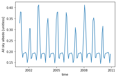
long_name and units for our new variable ASA, which is how xarray knew what to put in the y-axis label.
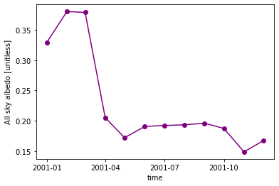
We can also just plot one year of data (2001) from the simulation, selecting the year using the .sel function. Note we also changed the color and marker for this plot.
More plotting examples are on the xarray web site
ds.ASA.sel(time='2001').plot(color="purple", marker="o") ;
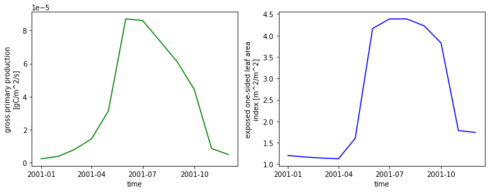
We can plot multiple graphs by using the keyword ax. Here, axes is an array we create consisting of a left and right axis created with plt.subplots.
fig, axes = plt.subplots(ncols=2, figsize=(10,4))
ds.GPP.sel(time='2001').plot(ax=axes[0], color='green')
ds.ELAI.sel(time='2001').plot(ax=axes[1], color='blue')
plt.tight_layout() ;
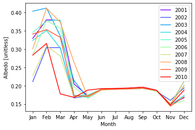
What if we wanted to compare years? We can start by creating columns for our years. The time.dt accessor allows us to access DateTime information. Next we will create a groupby object across our years. We will use this grouping to plot each year.
For more information about working with time in xarray, see the xarray documentation.
# create month and year columns
ds["year"] = ds.time.dt.year
ds["month_name"] = ds.time.dt.strftime("%b")

# group by year
groups = ds.groupby("year")

# plot each year
colors = plt.cm.rainbow(np.linspace(0, 1, 10))
for count, group in enumerate(groups):
    year = group[0]
    df = group[1]
    plt.plot(df.month_name, df.ASA, label=year, color=colors[count])
plt.legend(loc='upper right')
plt.xlabel("Month")
plt.ylabel("Albedo [unitless]") ;
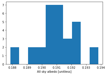
We can also plot a histogram across all years from the summer (June, July, and August). This is done by using .dt and the .isin accessors to subset the data (time.dt.month.isin([6, 7, 8])).
ds.ASA.isel(time=(ds.time.dt.month.isin([6, 7, 8]))).plot.hist() ;
3.2 Plotting in multiple dimensions#
When the data is two-dimensional, by default xarray calls xarray.plot.pcolormesh().
# pcolormesh plot
ds.sel(time='2001').H2OSOI.plot(x='time', yincrease=False, robust=True) ;
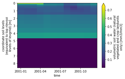
The depth to bedrock for this gridcell is ~ 4 meters, which means no soil moisture or soil temperature are calculated for deeper soil horizons.
You can see this by running the following code block, or entering it into the terminal (see zbedrock all the way at the end of the ncdump output):
!ncdump -v zbedrock /scratch/$USER/my_subset_data/surfdata_*
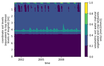
We can also make a contour plot:
ds.H2OSOI.plot.contourf(x='time', yincrease=False) ;
H2OSOI) for year 2001 as a linegraph, where each line is a different levsoi value? ( Hint: check out the hue parameter for plotting in xarray).
# plot your graph here
3.3 Visualizing Relationships#
Plotting can be useful for looking at relationships between different variables. What do you expect the relationship between latent heat flux and GPP to be? Below we are breaking up the data by season (time.dt.season is a built-in accessor).
ds["season"] = ds.time.dt.season
grouped = ds.groupby('season')
for key, group in grouped:
    plt.scatter(group.EFLX_LH_TOT, group.GPP, label=key)
plt.legend(loc="lower right")
plt.xlabel("Latent Heat Flux [W m$^{-2}$]")
plt.ylabel("GPP [gC m$^{-2}$ s$^{-1}$]") ;
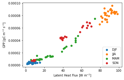
Questions:
How is albedo related to GPP?
How does this relationship play out over different seasons?
What other relationships can you elucidate from these simulations?
# plot some relationships here
4. Aggregating and averaging#
4.1 Basic aggregation methods#
Often we will want to aggregate our simulations from monthly to yearly or larger sums or averages. There are various ways to do this using xarray. A very common step would be to apply some function over the whole dataset, such as sum(), mean(), min(), or max(). Let’s explore some of these methods.
# compute the average GPP across the whole time series
# NOTE these values are not weighted by the number of days in each month.
ds.GPP.mean().values
array(3.610761e-05, dtype=float32)
Let’s also calculate the average GPP for a specific year, weighting by the number of days in each month and coverting to different units.
# calculate GPP for year 2005
# weight by the number of days in the month (non-leap years)
days_in_month = [31,28,31,30,31,30,31,31,30,31,30,31]
gpp_pm = ds.sel(time='2005').GPP*days_in_month/365.

# convert from GPP in gC/m^2/s to gC/m^2/year (x 60 seconds per minute x 60 minutes per hour x 24 hours per day x 365 days per year)
gpp_pm.sum().values * 86400. * 365.
1103.6826305738941
Can you find the maximum soil volumetric water content for the soil at 0.26 m?
# calculate answer here
4.2 Split-Apply-Combine#
You saw in our plotting above that we used xarray’s .groupby function to group our dataset by a specific variable (in that instance, years). This groupy operation allows us to aggregate our data conditionally on some coordinate label or group. This then allows us to perform split / apply / combine methods on xarray DataArrays and Datasets:
Splitting the dataset into groups based on some criteria
Applying a function to each of those groups (e.g. aggregating, performing a transform, or filtering)
Combining the results back into one data structure
Let’s use this methodology to remove seasonality from our dataset.
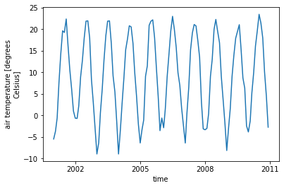
# calculate temperature in Celsius
ds['tair'] = ds.TBOT - 273.15
ds['tair'].attrs['units'] = 'degrees Celsius'
ds['tair'].attrs['long_name'] = 'air temperature'

# plot temperature across whole time series
ds.tair.plot() ;
First we will split the data by month:
ds.tair.groupby(ds.time.dt.month)
DataArrayGroupBy, grouped over 'month'
12 groups with labels 1, 2, 3, 4, 5, 6, 7, 8, 9, 10, 11, 12.
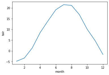
Now we can apply a calculation to each group - either an aggregation function, which will reduce the size of the group, or a transformation, which will preserve the group’s full size. Here we will take an average. Notice that the dimensions are now 1 x 12, because we have averaged across all years for each month.
# split-apply-combine
t_clim = ds.tair.groupby(ds.time.dt.month).mean()
t_clim
<xarray.DataArray 'tair' (month: 12)>
dask.array<stack, shape=(12,), dtype=float32, chunksize=(1,), chunktype=numpy.ndarray>
Coordinates:
  * month    (month) int64 1 2 3 4 5 6 7 8 9 10 11 12
t_clim.plot() ;
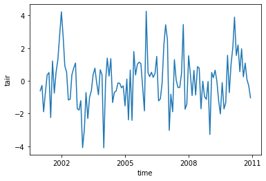
If we combine steps we can use these methods to remove the seasonality from our original dataset. Note here that the dataset is now 1 x 120 in dimension.
gb = ds.tair.groupby(ds.time.dt.month)
t_anom = gb - gb.mean(dim = 'time')
t_anom
<xarray.DataArray 'tair' (time: 120)>
dask.array<getitem, shape=(120,), dtype=float32, chunksize=(1,), chunktype=numpy.ndarray>
Coordinates:
  * time     (time) object 2001-01-01 00:00:00 ... 2010-12-01 00:00:00
month (time) int64 1 2 3 4 5 6 7 8 9 10 11 ... 2 3 4 5 6 7 8 9 10 11 12t_anom.plot() ;
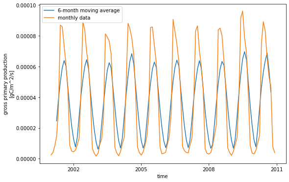
We can also calculate rolling means using the rolling function. Here we will calculate a 6-month rolling average of GPP.
mv_avg = ds.GPP.rolling(time=6, center=True).mean()
mv_avg.plot(size = 6)
ds.GPP.plot()
plt.legend(['6-month moving average', 'monthly data']) ;
# calculate value here