Chapter 3: Communication Primitives (Collective Operations)

Every distributed strategy from Chapter 2 boils down to a pattern of communication (collective operations) between GPUs. Once you understand these communication primitives, every distributed strategy is just a specific pattern of these operations.

This chapter covers the building blocks of distributed training: ranks, process groups, and the five collective operations you'll see throughout the guide.

Processes and Ranks

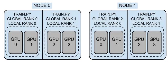
Distributed training runs multiple copies of your training script simultaneously -- one per GPU. Each copy is called a process, and each process has a unique identifier called a rank.

Each process is identified by three numbers (assigned by the launcher):

Term	Meaning	Range
WORLD_SIZE	Total number of processes	—
WORLD_RANK (or RANK)	Global ID of this process	0 to WORLD_SIZE-1
LOCAL_RANK	ID within this node	0 to GPUs_per_node-1

For example, with 2 nodes and 2 GPUs each, you have 4 processes with WORLD_RANKs 0-3. Each node has local LOCAL_RANKs 0-1. The LOCAL_RANK is used to assign a GPU to each process, while the WORLD_RANK is used for coordination (e.g., rank 0 handles logging and checkpointing). WORLD_SIZE is the total number of processes (4 in this example) and is used for scaling learning rates and calculating effective batch sizes.

Figure 1: World Rank vs Local Rank across two nodes with 4 GPUs each. (Source: [Medium](https://medium.com/red-buffer/getting-started-with-pytorch-distributed-54ae933bb9f0))

• You need to use LOCAL_RANK to assign a GPU: torch.cuda.set_device(LOCAL_RANK).
• You need to use WORLD_RANK for coordination: rank 0 typically handles logging, checkpointing, and data download.
• WORLD_SIZE is used for scaling learning rates and calculating effective batch sizes. For example, if your per-GPU batch size is 16 and you have WORLD_SIZE=4, your effective batch size is 16 × 4 = 64.

The above three variables are set by your launcher (e.g., torchrun, mpiexec, mpirun) when you start your distributed job. The launcher ensures that each process gets the correct rank and world size, allowing them to coordinate properly.

Launchers

To start a distributed training job, you use a launcher that spawns multiple processes with the appropriate environment variables set.

The most common launchers are:

Launcher	Use for	Example Command
torchrun	Single-node multi-GPU	torchrun --nproc_per_node=4 train.py
mpiexec or mpirun	Multi-node	mpiexec -n 8 --ppn 4 --cpu-bind none python train.py

You can also use mpiexec + torchrun for multi-node training, but this requires additional setup to ensure that the environment variables are correctly propagated across nodes.

torchrun -- Single Node Multi-GPU Training

torchrun is the recommended launcher for single-node multi-GPU training. It automatically sets LOCAL_RANK, WORLD_RANK, and WORLD_SIZE for each process.

For example, if you have 4 GPUs on a single node, you can launch your training script with:

torchrun --nproc_per_node=4 train.py

This will start 4 processes, each with LOCAL_RANK 0-3 and WORLD_RANK 0-3, and WORLD_SIZE 4.

For multi-node training, using torchrun requires additional setup to ensure that the environment variables are correctly propagated across nodes. This can be done with the --rdzv_backend and --rdzv_endpoint options, but it is often simpler to use mpiexec for multi-node training.

Essentially, you have to run torchrun on each node, and ensure that the WORLD_RANK and WORLD_SIZE are correctly set across nodes. It will look something like this:

# On Node 1 -- (the master node)
torchrun --nodes 2
    --nproc_per_node=4 \
    --node_rank=0 \
    --master_addr=node1 \ # IP or hostname of the master node
    --master_port=29500 \
    train.py    

# On Node 2 -- (the worker node)
torchrun --nodes 2
    --nproc_per_node=4 \
    --node_rank=1 \
    --master_addr=node1 \ # IP or hostname of the master node
    --master_port=29500 \
    train.py

The above setup can be error-prone, which is why using mpiexec or mpirun for multi-node training is often recommended, as it handles the multi-node coordination for you.

mpiexec or mpirun -- Multi-Node Training

For multi-node training, mpiexec (or mpirun) is the most common launcher. It uses MPI to launch one process per GPU across multiple nodes and sets the appropriate environment variables for each process. For example, if you have 2 nodes with 4 GPUs each (8 total), you can launch your training script with:

mpiexec -n 8 --ppn 4 --cpu-bind none python train.py

But you need to ensure that your training script correctly initializes the process group and sets the device based on the environment variables set by your MPI flavor (e.g., OpenMPI, Cray MPICH).

The utils/distributed.py file in this repository provides a setup_distributed() function that abstracts away the details of initializing the process group and setting the device, making it easier to write distributed training scripts that can work with different launchers, such as torchrun, OpenMPI, or Cray MPICH.

This table summarizes the launchers and their environment variable handling:

Launcher	WORLD_RANK	LOCAL_RANK	WORLD_SIZE
torchrun	RANK	LOCAL_RANK	WORLD_SIZE
OpenMPI	OMPI_COMM_WORLD_RANK	OMPI_COMM_WORLD_LOCAL_RANK	OMPI_COMM_WORLD_SIZE
Cray MPICH	PMI_RANK	PMI_LOCAL_RANK	PMI_SIZE

Process Groups

A process group is a set of ranks that communicate together. When you call init_process_group(), it creates the default group containing all ranks:

import torch.distributed as dist

dist.init_process_group(backend="nccl")  # all ranks join

# All ranks can now communicate with each other
dist.all_reduce(tensor)  # works across all ranks

Sometimes you need only some ranks to communicate. This is common in hybrid parallelism (e.g., FSDP within nodes, DDP across nodes). In that case, you create subgroups:

# Create a subgroup for ranks 0-3 (e.g., for TP within nodee 1)
tp_group = dist.new_group(ranks=[0, 1, 2, 3])

# Create a subgroup for ranks 4-7 (e.g., for TP within node 2)
tp_group_2 = dist.new_group(ranks=[4, 5, 6, 7])

Backends

A backend is the communication layer used by PyTorch to exchange data between processes (e.g., GPUs or nodes). Different backends are optimized for different hardware and use cases. The table below summarizes the common backends that pyTorch supports:

Backend	Hardware	Typical Use Case
nccl	NVIDIA GPUs	High-performance GPU training (default)
gloo	CPU	CPU training or fallback
mpi	CPU / GPU	MPI-based environments and launchers

Tip

For GPU training, nccl is almost always the best choice due to its optimized collective communication (e.g., all-reduce, broadcast).

Notes for Derecho

On Derecho, you should use nccl for GPU communication. However, proper performance depends on having the correct environment and network configuration.

• Derecho uses Cray HPE Slingshot, which requires NCCL to be built or configured with Slingshot support.
• The PyTorch wheel provided in your environment.yaml in this repo includes NCCL support compatible with Slingshot 11.
• You should verify that:
  • The correct NCCL library is being used at runtime
  • Environment variables (e.g., networking and transport settings) are properly configured
  • The runtime is not falling back to a slower backend (e.g., gloo)

Warning

Misconfigured NCCL environments can silently degrade performance significantly (e.g., falling back to TCP instead of high-speed interconnects).

---

The Most Common Collective Operations

Collective operations (or "collectives") are communication patterns where multiple ranks participate together. Every distributed training strategy is built from these primitives.

The NVIDIA NCCL library provides highly optimized implementations of these collectives for GPU communication. You can find more details in the NCCL documentation.

The most common collectives you'll see in distributed training are:

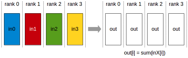
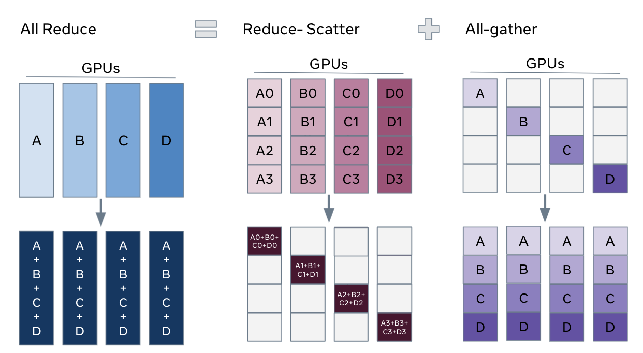
1. All-Reduce

Every GPU starts with a value. After all-reduce operations, every GPU has the sum (or average, min, max) of all values across GPUs.

all-reduce is the core of DDP, where gradients are all-reduced after each backward pass to compute the average gradient across all GPUs before the optimizer step.

Figure 2: All-Reduce — every GPU ends up with the sum of all values. (Source: NVIDIA NCCL documentation)

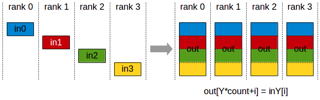
2. All-Gather

Each GPU has a piece of data. After all-gather, every GPU has all the pieces concatenated.

FSDP uses this to reassemble sharded parameters before forward/backward passes, and TP uses it to gather sharded activations across GPUs.

Figure 3: All-Gather — each GPU contributes a piece, and every GPU ends up with all pieces concatenated. (Source: NVIDIA NCCL documentation)

Before:           Operation:         After:
GPU 0: [A]                          GPU 0: [A, B, C, D]
GPU 1: [B]     ── all-gather ──►    GPU 1: [A, B, C, D]
GPU 2: [C]                          GPU 2: [A, B, C, D]
GPU 3: [D]                          GPU 3: [A, B, C, D]

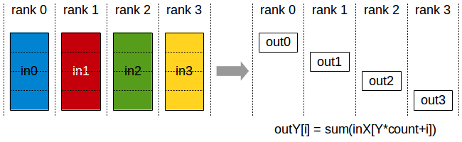
3. Reduce-Scatter

Reduce-Scatter is the inverse of all-gather. It reduces (sums) data and scatters the result so each GPU gets one piece.

FSDP uses this after backward to produce sharded gradients.

Figure 4: Reduce-Scatter — data is reduced (summed) and each GPU receives one shard of the result. (Source: NVIDIA NCCL documentation)

Before:                    Operation:              After:
GPU 0: [a0, a1, a2, a3]                          GPU 0: [a0+b0+c0+d0]
GPU 1: [b0, b1, b2, b3]  ── reduce-scatter ──►   GPU 1: [a1+b1+c1+d1]
GPU 2: [c0, c1, c2, c3]      (sum)               GPU 2: [a2+b2+c2+d2]
GPU 3: [d0, d1, d2, d3]                          GPU 3: [a3+b3+c3+d3]

All-Gather + Reduce-Scatter Pattern

The all-gather + reduce-scatter pair is a powerful pattern for sharding tensors across GPUs while still supporting global computation.

FSDP uses this pattern to shard model states: it all-gathers parameter shards before forward/backward computation and reduce-scatters gradients during the backward pass.
In tensor-parallel training, similar all-gather / reduce-scatter patterns are also used in some variants—especially sequence parallelism and related activation-sharding schemes.

Figure 5: FSDP uses all-gather to materialize parameters for computation and reduce-scatter to return gradients to sharded form. (Source: PyTorch/FSDP documentation and Meta FSDP materials)

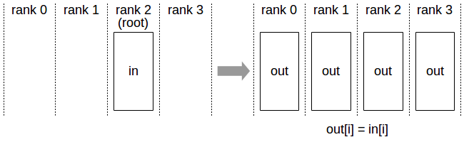
4. Broadcast

The Broadcast operation copies an N-element buffer from the root rank to all the ranks. So one GPU sends its data to all others as shown in the image below....

Used for syncing initial model weights or distributing hyperparameters.

Figure 6: Broadcast — one GPU sends its data to all other GPUs. (Source: NVIDIA NCCL documentation)

Before:           Operation:         After:
GPU 0: [X]                          GPU 0: [X]
GPU 1: [ ]     ── broadcast ──►     GPU 1: [X]
GPU 2: [ ]        (from 0)          GPU 2: [X]
GPU 3: [ ]                          GPU 3: [X]

5. Point-to-Point (Send/Recv)

Direct communication between two specific GPUs. Pipeline parallelism uses this: stage N sends activations to stage N+1.

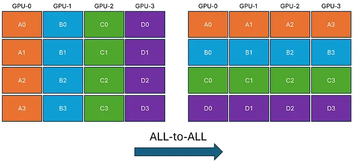
6. All-to-All

In All-to-All, each GPU transmits unique data to every other GPU. To achieve this, each GPU breaks down its data into chunks. Subsequently, each GPU directly sends and receives these chunks to and from every other GPU. Finally, each GPU reconstructs the received data chunks.

Figure 7: All-to-All — each GPU sends unique data chunks to every other GPU.

Hardware Topology Matters

The speed of these collective operations depends entirely on the hardware connecting your GPUs. On virtually all modern supercomputers, intra-node communication (GPUs within the same node, connected via NVLink) is orders of magnitude faster than inter-node communication (GPUs across different nodes, connected via network fabrics like InfiniBand or Slingshot).

This physical reality dictates how you map your distributed strategy to the hardware.

For example, on NCAR's Derecho system (which has 4× A100 GPUs per node):

• Within a node (High Bandwidth): Use communication-heavy, latency-sensitive strategies like Tensor Parallelism (TP) or Sequence Parallelism. These require constant, blocking data transfers during the forward and backward passes and must utilize NVLink.
• Across nodes (Lower Bandwidth): Use bandwidth-efficient strategies like FSDP or DDP. These strategies are designed to hide network latency by overlapping their communication (like gradient synchronization) with the ongoing computation of the backward pass.

See the Derecho Guide for full hardware specs.

Hands-On: Try the Primitives

The tests/ directory has scripts that let you run these operations directly:

• tests/all_reduce_test.py — run an all-reduce and verify the result
• tests/send_recv_test.py — point-to-point communication between ranks
• tests/torch_comm_bench.py — benchmark all-reduce, broadcast, and send/recv at various tensor sizes

# Run on 4 GPUs
mpiexec -n 4 --ppn 4 --cpu-bind none python tests/all_reduce_test.py

Also, see nccl-tests for more comprehensive benchmarks of NCCL collectives.

What's Next?

Now that you understand the communication building blocks, Chapter 4 puts them to use with the simplest and most common distributed strategy, ie.e. Data Parallel (DDP).

Next: Chapter 4 — Data Parallel (DDP)